

The main Curvature KML files are colored on a spectrum to help you identify the overall twistiness of roads (or multi-mile sections of curves in the case of roads with a mixture of straight and curvy sections). Curvature also produces KML files called “Detected Curves” (which are appended with “.curves” at the end of the file name) instead show you every single segment of a curvy road colored according to its curve radius as shown here:
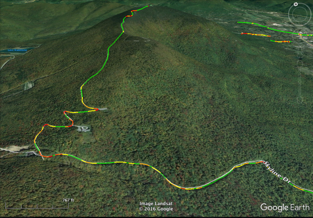
- Green – Straight or large-radius curves which are considered “straight.” Radius: > 175 meters
- Yellow – Broad, sweeping turns. Radius: 100 m – 175 m
- Light Orange – Medium turns. Radius: 60 m – 100 m
- Dark Orange – Tight turns. Radius: 25 m – 60 m
- Red – Super-tight turns. Radius: ≤ 25 meters
These “Detected Curves” files can take a lot of processing power for Google Earth to render and may not work well on all computers for large regions, especially when zoomed way out. One trick to get them to render is to open Google Earth and zoom in so that your view is only a few tens of miles across — not a whole state or country. Once you are zoomed in, then open or enable the “[file name].curves.kmz” layer and click quickly to prevent Google Earth from zooming out to the full region extent. Since it is only showing a small number of lines, the rendering requirements are lower and it shouldn’t crash Google Earth.
Viewing challenges aside, the “Detected Curves” files will show you how Curvature is interpreting the road data and what curves it finds in the data. Sometimes roads that we know to be relatively straight will show up with strangely high curvature values. Looking at the road in the “Detected Curves” file will highlight the curves in the data, which may be real or imaginary.
Take for example this street in Seattle, WA: Sand Point Way NE. The road is straight, but the way divided and undivided sections of the road are mapped, it looks to the curvature program like the road is twisting back and forth.
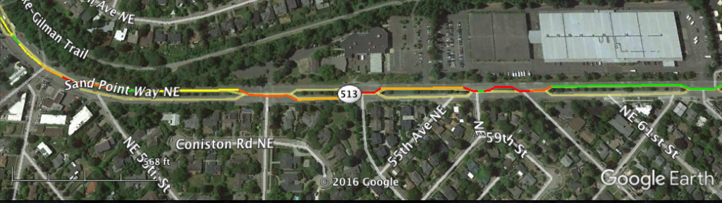
A similar effect can be seen when roads are imported from noisy GPS traces that jiggle back and forth across the road width, presenting curves that don’t exist in reality. Unlike the divided/undivided roads, these jiggles can be edited out in OpenStreetMap to remove the phantom curves.